Tuesday, 22 December 2015

Analyzing AWR reports for oracle

AWR report generates the performance statistics related to database server like system and session statistics, segment usage statistics, resource intensive SQLs, time model statistics and buffer cache details.

The important sections in the report are given below. For better understanding a snap from AWR for each section is provided here. 

  • Elapsed Time
  • Top 5 timed events
  • SQL statistics
  • Time Model Statistics
1. Elapsed Time

Elapsed time is the difference between begin snap time and end snap time. This time should be equal to the time for which the load test is performed for desired load. If DB time is less than elapsed time, it can be concluded that the bottleneck is not there in the database, else further analysis is required to ascertain the database performance bottleneck.

upload_2015-4-30_10-1-46.png 

2. Top 5 timed events

This section can be interpreted as top 5 bottlenecks in database. All other sections in the report will provide breakup of these 5 timed events in to different metrics such as SQL Statistics, IO Statistics, Buffer Pool Statistics and Segment Statistics etc. Most of the database performance bottlenecks should get resolved if these top 5 events are eliminated or reduced.

upload_2015-4-30_10-2-41.png 

3. SQL Statistics
This section provides the details of the SQL queries that are executed in the database during the test performed under load. Generally primary concern from Performance point of view for the application is the response times of the transactions at the peak load. This section address the issues related to response times of the database queries. Main points to look under this section are

SQL Ordered by Elapsed Time: Includes SQL statements that took significant execution time during processing.

SQL Ordered by CPU Time: Includes SQL statements that consumed significant database server CPU time during its processing. Examples of Server CPU time are Sorting, Hashing.

SQL Ordered by Gets: SQLs performed a high number of logical reads (from the cache) while retrieving data.

SQL Ordered by Reads: SQLs performed a high number of physical disk reads while retrieving data.

SQL Ordered by Parse Calls: These SQLs experienced a high number of parsing operations.

SQL Ordered by Executions: Lists the number of executions happened of each SQL.

4. Time Model Statistics
This section gives split up of time spent by the application in the processing of SQL queries like PL/SQL processing time, parsing, sequence load, sql execution etc.

  • DB CPU: total CPU time consumed by database, apart from CPU background processes, in snapshot interval.
  • sql execute elapsed time: Time spent by all SQL statements to execute
  • DB time: Total time spent in DB, apart from time spent by background processes.

Automatic Database Diagnostic Monitor (ADDM) in Oracle Database 10g:

Overview
The Automatic Database Diagnostic Monitor (ADDM) analyzes data in the Automatic Workload Repository (AWR) to identify potential performance bottlenecks. For each of the identified issues it locates the root cause and provides recommendations for correcting the problem. An ADDM analysis task is performed and its findings and recommendations stored in the database every time an AWR snapshot is taken provided the STATISTICS_LEVEL parameter is set to TYPICAL or ALL. The ADDM analysis includes the following.
  • CPU load
  • Memory usage
  • I/O usage
  • Resource intensive SQL
  • Resource intensive PL/SQL and Java
  • RAC issues
  • Application issues
  • Database configuration issues
  • Concurrency issues
  • Object contention
There are several ways to produce reports from the ADDM analysis which will be explained later, but all follow the same format. The findings (problems) are listed in order of potential impact on database performance, along with recommendations to resolve the issue and the symptoms which lead to it's discovery. An example from my test instance is shown below.
FINDING 1: 59% impact (944 seconds)
-----------------------------------
The buffer cache was undersized causing significant additional read I/O.

   RECOMMENDATION 1: DB Configuration, 59% benefit (944 seconds)
      ACTION: Increase SGA target size by increasing the value of parameter
         "sga_target" by 28 M.

   SYMPTOMS THAT LED TO THE FINDING:
      Wait class "User I/O" was consuming significant database time. (83%
      impact [1336 seconds])
The recommendations may include:
  • Hardware changes
  • Database configuration changes
  • Schema changes
  • Application changes
  • Using other advisors
The analysis of I/O performance is affected by the DBIO_EXPECTED parameter which should be set to the average time (in microseconds) it takes to read a single database block from disk. Typical values range from 5000 to 20000 microsoconds. The parameter can be set using the following.
EXECUTE DBMS_ADVISOR.set_default_task_parameter('ADDM', 'DBIO_EXPECTED', 8000);

Enterprise Manager
The obvious place to start viewing ADDM reports is Enterprise Manager. The "Performance Analysis" section on the "Home" page is a list of the top five findings from the last ADDM analysis task.
Specific reports can be produced by clicking on the "Advisor Central" link, then the "ADDM" link. The resulting page allows you to select a start and end snapshot, create an ADDM task and display the resulting report by clicking on a few links.

addmrpt.sql Script
The addmrpt.sql script can be used to create an ADDM report from SQL*Plus. The script is called as follows.
-- UNIX
@/u01/app/oracle/product/10.1.0/db_1/rdbms/admin/addmrpt.sql

-- Windows
@d:\oracle\product\10.1.0\db_1\rdbms\admin\addmrpt.sql
It then lists all available snapshots and prompts you to enter the start and end snapshot along with the report name.
An example of the ADDM report can be seen here.

DBMS_ADVISOR
The DBMS_ADVISOR package can be used to create and execute any advisor tasks, including ADDM tasks. The following example shows how it is used to create, execute and display a typical ADDM report.
BEGIN
  -- Create an ADDM task.
  DBMS_ADVISOR.create_task (
    advisor_name      => 'ADDM',
    task_name         => '970_1032_AWR_SNAPSHOT',
    task_desc         => 'Advisor for snapshots 970 to 1032.');

  -- Set the start and end snapshots.
  DBMS_ADVISOR.set_task_parameter (
    task_name => '970_1032_AWR_SNAPSHOT',
    parameter => 'START_SNAPSHOT',
    value     => 970);

  DBMS_ADVISOR.set_task_parameter (
    task_name => '970_1032_AWR_SNAPSHOT',
    parameter => 'END_SNAPSHOT',
    value     => 1032);

  -- Execute the task.
  DBMS_ADVISOR.execute_task(task_name => '970_1032_AWR_SNAPSHOT');
END;
/

-- Display the report.
SET LONG 1000000 LONGCHUNKSIZE 1000000
SET LINESIZE 1000 PAGESIZE 0
SET TRIM ON TRIMSPOOL ON
SET ECHO OFF FEEDBACK OFF

SELECT DBMS_ADVISOR.get_task_report('970_1032_AWR_SNAPSHOT') AS report
FROM   dual;

SET PAGESIZE 24
The value for the SET LONG command should be adjusted to allow the whole report to be displayed.
The relevant AWR snapshots can be identified using the DBA_HIST_SNAPSHOT view.

Related Views
The following views can be used to display the ADDM output without using Enterprise Manager or the GET_TASK_REPORT function.
  • DBA_ADVISOR_TASKS - Basic information about existing tasks.
  • DBA_ADVISOR_LOG - Status information about existing tasks.
  • DBA_ADVISOR_FINDINGS - Findings identified for an existing task.
  • DBA_ADVISOR_RECOMMENDATIONS - Recommendations for the problems identified by an existing task.

SQL Developer and ADDM Reports
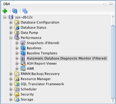
If you are using SQL Developer 4 onward, you can view ADDM reports directly from SQL Developer. If it is not already showing, open the DBA pane "View > DBA", expand the connection of interest, then expand the "Performance" node. The ADDM reports are available from the "Automatic Database Diagnostics Monitor" node.
SQL Developer - ADDM Report

Jboss Configuration For Best Performance

Monday, 21 December 2015

Calculating Concurrency from Performance Test Results

Number of Items in the system = Arrival Rate x Response Time

To apply little law to a performance test we must first make sure that we are taking measurements from when the system under test is balanced. Remember a balanced system the rate of work entering the system matches the rate of work leaving the system. This for a typical load testing tool is after the ramp up period and the number of virtual users remains constant and response times have stabilised and the transaction per second graph is level. To capture this period of time in LoadRunner for example you would need to select the time period in the Summary report filter or under the Tools -> Options.
So record the average response time for the transaction of interest and the number of times per second the transaction is executed.
performanceresponsetimes
So from the example above the response time is 43.613 seconds. The arrival rate is the number of transactions executed divided by the duration. The duration for this example was a 10 minute period as can be confirm by the LoadRunner summary below.
LoadRunner Performance Testv Duration
This gives you an arrival rate of 2.005 calculated by taking the count 1203 divided by the duration 600.
So the concurrent number of users waiting for a search to return is 87.44
There you go from your performance test results you can easily calculate the concurrency for a particular transaction.

Sunday, 20 December 2015

HOW GARBAGE COLLECTION WORKS IN JAVA

The important things about the garbage collections are

1) objects are created on heap in Java irrespective of there scope e.g. local or member variable. while its worth noting that class variables or static members are created in method area of Java memory space and both heap and method area is shared between different thread.
2) Garbage collection is a mechanism provided by Java Virtual Machine to reclaim heap space from objects which are eligible for Garbage collection.
3) Garbage collection relieves java programmer from memory management which is essential part of C++ programming and gives more time to focus on business logic.
4) Garbage Collection in Java is carried by a daemon thread called Garbage Collector.
5) Before removing an object from memory Garbage collection thread invokes finalize () method of that object and gives an opportunity to perform any sort of cleanup required.
6) You as Java programmer can not force Garbage collection in Java; it will only trigger if JVM thinks it needs a garbage collection based on Java heap size.
7) There are methods like System.gc () and Runtime.gc () which is used to send request of Garbage collection to JVM but it’s not guaranteed that garbage collection will happen.
8) If there is no memory space for creating new object in Heap Java Virtual Machine throws OutOfMemoryError or java.lang.OutOfMemoryError heap space
9) J2SE 5(Java 2 Standard Edition) adds a new feature called Ergonomics goal of ergonomics is to provide good performance from the JVM with minimum of command line tuning.

When an Object becomes Eligible for Garbage Collection
An Object becomes eligible for Garbage collection or GC if its not reachable from any live threads or any static refrences in other words you can say that an object becomes eligible for garbage collection if its all references are null. Cyclic dependencies are not counted as reference so if Object A has reference of object B and object B has reference of Object A and they don't have any other live reference then both Objects A and B will be eligible for Garbage collection.
Generally an object becomes eligible for garbage collection in Java on following cases:
1) All references of that object explicitly set to null e.g. object = null
2) Object is created inside a block and reference goes out scope once control exit that block.
3) Parent object set to null, if an object holds reference of another object and when you set container object's reference null, child or contained object automatically becomes eligible for garbage collection.
4) If an object has only live references via WeakHashMap it will be eligible for garbage collection. To learn more about HashMap see here How HashMap works in Java.

Heap Generations for Garbage Collection in JavaJava objects are created in Heap and Heap is divided into three parts or generations for sake of garbage collection in Java, these are called as Young generation, Tenured or Old Generation and Perm Area of heap.
New Generation is further divided into three parts known as Eden space, Survivor 1 and Survivor 2 space. When an object first created in heap its gets created in new generation inside Eden space and after subsequent Minor Garbage collection if object survives its gets moved to survivor 1 and then Survivor 2 before Major Garbage collection moved that object to Old or tenured generation.

Permanent generation of Heap or Perm Area of Heap is somewhat special and it is used to store Meta data related to classes and method in JVM, it also hosts String pool provided by JVM as discussed in my string tutorial why String is immutable in Java. There are many opinions around whether garbage collection in Java happens in perm area of java heap or not, as per my knowledge this is something which is JVM dependent and happens at least in Sun's implementation of JVM. You can also try this by just creating millions of String and watching for Garbage collection or OutOfMemoryError.

Types of Garbage Collector in JavaJava Runtime (J2SE 5) provides various types of Garbage collection in Java which you can choose based upon your application's performance requirement. Java 5 adds three additional garbage collectors except serial garbage collector. Each is generational garbage collector which has been implemented to increase throughput of the application or to reduce garbage collection pause times.

1) Throughput Garbage Collector: This garbage collector in Java uses a parallel version of the young generation collector. It is used if the -XX:+UseParallelGC option is passed to the JVM via command line options . The tenured generation collector is same as the serial collector.

2) Concurrent low pause Collector: This Collector is used if the -Xingc or -XX:+UseConcMarkSweepGC is passed on the command line. This is also referred as Concurrent Mark Sweep Garbage collector. The concurrent collector is used to collect the tenured generation and does most of the collection concurrently with the execution of the application. The application is paused for short periods during the collection. A parallel version of the young generation copying collector is sued with the concurrent collector. Concurrent Mark Sweep Garbage collector is most widely used garbage collector in java and it uses algorithm to first mark object which needs to collected when garbage collection triggers.

3) The Incremental (Sometimes called train) low pause collector: This collector is used only if -XX:+UseTrainGC is passed on the command line. This garbage collector has not changed since the java 1.4.2 and is currently not under active development. It will not be supported in future releases so avoid using this and please see 1.4.2 GC Tuning document for information on this collector.
Important point to not is that -XX:+UseParallelGC should not be used with -XX:+UseConcMarkSweepGC. The argument passing in the J2SE platform starting with version 1.4.2 should only allow legal combination of command line options for garbage collector but earlier releases may not find or detect all illegal combination and the results for illegal combination are unpredictable. It’s not recommended to use this garbage collector in java.

JVM Parameters for garbage collection in JavaGarbage collection tuning is a long exercise and requires lot of profiling of application and patience to get it right. While working with High volume low latency Electronic trading system I have worked with some of the project where we need to increase the performance of Java application by profiling and finding what causing full GC and I found that Garbage collection tuning largely depends on application profile, what kind of object application has and what are there average lifetime etc. for example if an application has too many short lived object then making Eden space wide enough or larger will reduces number of minor collections. you can also control size of both young and Tenured generation using JVM parameters for example setting -XX:NewRatio=3 means that the ratio among the young and tenured generation is 1:3 , you got to be careful on sizing these generation. As making young generation larger will reduce size of tenured generation which will force Major collection to occur more frequently which pauses application thread during that duration results in degraded or reduced throughput. The parameters NewSize and MaxNewSize are used to specify the young generation size from below and above. Setting these equal to one another fixes the young generation. In my opinion before doing garbage collection tuning detailed understanding of garbage collection in java is must and I would recommend reading Garbage collection document provided by Sun Microsystems for detail knowledge of garbage collection in Java. Also to get a full list of JVM parameters for a particular Java Virtual machine please refer official documents on garbage collection in Java. I found this link quite helpful though http://www.oracle.com/technetwork/java/gc-tuning-5-138395.html

Full GC and Concurrent Garbage Collection in JavaConcurrent garbage collector in java uses a single garbage collector thread that runs concurrently with the application threads with the goal of completing the collection of the tenured generation before it becomes full. In normal operation, the concurrent garbage collector is able to do most of its work with the application threads still running, so only brief pauses are seen by the application threads. As a fall back, if the concurrent garbage collector is unable to finish before the tenured generation fill up, the application is paused and the collection is completed with all the application threads stopped. Such Collections with the application stopped are referred as full garbage collections or full GC and are a sign that some adjustments need to be made to the concurrent collection parameters. Always try to avoid or minimize full garbage collection or Full GC because it affects performance of Java application. When you work in finance domain for electronic trading platform and with high volume low latency systems performance of java application becomes extremely critical an you definitely like to avoid full GC during trading period.

Summary on Garbage collection in Java1) Java Heap is divided into three generation for sake of garbage collection. These are young generation, tenured or old generation and Perm area.
2) New objects are created into young generation and subsequently moved to old generation.
3) String pool is created in Perm area of Heap, garbage collection can occur in perm space but depends upon JVM to JVM.
4) Minor garbage collection is used to move object from Eden space to Survivor 1 and Survivor 2 space and Major collection is used to move object from young to tenured generation.
5) Whenever Major garbage collection occurs application threads stops during that period which will reduce application’s performance and throughput.
6) There are few performance improvement has been applied in garbage collection in java 6 and we usually use JRE 1.6.20 for running our application.
7) JVM command line options –Xmx and -Xms is used to setup starting and max size for Java Heap. Ideal ratio of this parameter is either 1:1 or 1:1.5 based upon my experience for example you can have either both –Xmx and –Xms as 1GB or –Xms 1.2 GB and 1.8 GB.
8) There is no manual way of doing garbage collection in Java.


VUser Calculations

Calculating How Many Maximum Number Of Users Required If We Need To Achieve 12K Transactions With SLA Of 5 Minutes

Total Number of Transactions to be completed = 12,000
Average Response Time = 5 Minutes

To avoid putting much load on the system I will add 5 Minutes so that to total time taken to complete one iteration will be 10 Minutes. This addition will include the thinktime between the each screen/transaction traverse.

Now, I know each iteration will take 10 Minutes to complete, hence in 60 Minutes only 6 transactions can be completed. i.e. 1 User will do 6 transactions in an hour.

Now how to calculate how many users are required to complete 12,000 transactions in an hour?
The calculation will be:
#Users Required = 12,000/6
= 2000 Users

This way we can find the number of users required if total throughput is provided with an average response time.

Hence to achieve 12,000 transactions I need 2000 Users with 5 minutes of thinktime in between the iterations with an average response time of 5 Minutes.


PACING Calculation

Pacing Calculation :

D = Duration of the test(test window/time frame)

B = Baseline time(total time taken by 1 Vu to complete 1 whole iteration)

T = Total amount of Think time in the script

I = Expected/Target iteration

R = Residual time of the test window.

R = ( D - (T + B)*I)

P = Pacing interval

Dividing the residual time by target iteration gives pacing interval

Hence:

P = R/I

D is pacing time.
(T + B)*I represents the duration of a scenario
and P is the waiting time before the next scenario

Calculating Pacing Time/Think Time to achieve 50 TPS with an average response time of 0.5 seconds with total of 100 Users
Let us start with calculating total number of transactions in an hour.
1 sec = 50 trnx
3600 sec = x
x = 3600 * 50 = 180000 trnx/hour by 100 Users

We have total number of users given as 100. Let us see how to calculate how many transactions each user will perform.
Total Number of Users = 100
Each User will perform 180000/100=1800 transactions/hour

Since, every transaction is taking on an average 0.5 seconds, let us see how much time is required to complete the each user transactions.
To complete 1800 trnx it will take 1800*0.5 = 15 minutes

So now, let us see how much think-time is required to complete the required number transactions per User in an hour.
1800 transactions will complete in 15 minutes
hence, 45 minutes of thinktime is required in between 1800 transactions (i.e. 45*60 = 2700 seconds of thinktime required in between 1800 transactions (per user))
2700 seconds = 1800 trnx
x = 1 trnx
x = 1.5 seconds think time need to include

Let us see how much time is required to complete each iteration.
Total time required to complete each Iteration = x + 0.5 seconds
= 1.5 + 0.5
= 2 seconds

Verification: Let us verify if our above calculation is correct.
Total time = 1800 * 2
= 3600 seconds
= 1 Hr

So, Each User will perform 1800 transactions where we will provide 2 seconds for each Iteration to complete.

Random Virtual User Pacing in LoadRunner:
I guess there's always a first time. I had never used LoadRunner's random virtual user (VU) pacing earlier, but am working on a project that will need to use this feature for the first time. And as I thought about it a little more, I may start using it more frequently now. Here's how it happened

This is one of the rare projects that provided me with excellent documentation - not only system documentation like the system specs, API Guides etc but also performance requirements like actual production volume reports and capacity models that estimated the projected volumes.

The capacity models estimated the maximum transaction load by hour as well as by minute (max TPM). What I needed to do was take maximum hourly load, divide it by 60 to get a per minute transactional load and use this as the average TPM. The idea was to vary the VU pacing so that over the whole duration of test, average load stays at this Average TPM but it also reaches the Max TPM randomly.

For example, if the maximum hourly transaction rate is 720 requests and maximum TPM is 20, the average TPM will be 720/60 = 12 and I will need to vary the pacing so that the load varies between 4TPM and 20TPM and averages to around 12TPM.
The Calculation:
To vary the transactional load, We knew we had to vary the VU Pacing randomly. Taking above example, I had to achieve 12TPM and I knew the transactions were taking around 1-2 seconds to complete. So I could have the pacing of around 120 seconds if I needed to generate a fixed load of 12TPM with a 5 second Ramp-up and 24 users.

ScriptTPMNumber of VUsPacing (sec)Ramp Up
Script 112241201 VU/5sec

So now to vary the TPM to x with the same 24 virtual users, I will need to have a pacing of 24*60/x. I got this from an old-fashioned logic which goes in my head this way:
24 users with a pacing of 60 seconds generate a TPM of 24
24 users with a pacing of 120 seconds generate a TPM of 24 * 60/120
24 users with a pacing of x seconds generate a TPM of 24 * 60/x

So using above formula, to vary the load from 20 to 4TPM I will need to vary the VU pacing from 72 to 360. So now we have:
ScriptTPMNumber of VUsPacing (sec)Ramp Up
Script 14 to 2024Random (72 to 360)1 VU/5sec


Of course, there's a caveat. The range of 72 to 360 seconds has an arithmetic mean of 216. 120 is actually the harmonic mean of the 2 numbers. So the actual variation in TPM will depend on the distribution of random numbers that LoadRunner generates within the given range. If it generates the numbers with a uniform distribution around the arithmetic mean of the range, then we have a problem.

I ran a quick test to find this out. I created an LR script and used the rand() function to generate 1000 numbers between the range with the assumption that LR uses a similar function to generate the random pacing values.

int i;
srand(time(NULL));
for (i=0;i<1000 br="" i="">lr_output_message("%d\n", rand() % 289 + 72);
}

And of course, the average came out close to the arithmetic mean of 72 and 360, which is 216.

So with the assumption that the function used by LoadRunner for generating random pacing values generates numbers that are uniformly distributed around the arithmetic mean of the range, we'll need to modify the range of pacing values so that the arithmetic mean of the range gives us the arithmetic mean of the TPM that we want...phew. What it means is that the above pacing values need to be modified from 72 to 360 (arithmetic mean = 216) to 72 to 168 (arithmetic mean = 120). However, this gives us the TPM range of 20 to 8.6 TPM with a harmonic mean of 12TPM.

But I'll live with it. I would rather have the average load stay around 12TPM. So here are the new values. Note the asterisk on TPM. I need to mention in the test plan that the actual TPM will vary from 8.6 to 20TPM with an average of 12TPM.

ScriptTPM*Number of VUsPacing (sec)Ramp Up
Script 14 to 2024Random (72 to 168)1 VU/5sec

Tuesday, 15 December 2015

IIS Configuration For Best Performance

Common Problem areas in IIS Performance are 

  1. Memory leak
  2. Thread Limit
  3. High cpu usage
  4. Cache
  5. HTTP compression
  6. Connection limtation
Configuration to improve IIS performance

Internet Information Services (IIS) exposes numerous configuration parameters that affect IIS performance. The following points describes several of these parameters and provides general guidance for setting the parameter values to improve IIS performance.

  • Configure Logging option(Log only essential information or completely disable IIS logging)
  • Disable IIS ASP debugging in production environments
  • Tune the value of the ASP Threads Per Processor Limit property
  • Tune the value of the ASP Queue Length property
  • Tune the MaxPoolThreads registry entry
  • Configure ASP.NET 2.0 MaxConcurrentRequests for IIS 7.5/7.0 Integrated mode
  • Enabling CPU Monitoring in IIS
  • Improving IIS Scalability and Availability with Network Load Balancing
  • Enable IIS HTTP compression
  • Configure HTTP expires header
  • Enable Output caching
  • Connection Limit in IIS
upload_2015-12-15_10-18-56.png

Configure Logging option(Log only essential information or completely disable IIS logging

With default settings, IIS logs almost everything under the hood . which results memory consumption and increase the response time . so to consume less memory You either can disable logging option or can select a number of essential events to log in your server. To disable logging follow these steps:

1. Click Start, point to All Programs, click Administrative Tools, and then click Internet Information Services (IIS) Manager.

2. In the Connections pane, click to expand Sites, click to select the Web site for which you would like to disable logging, click to select Features View, and then double-click the Logging feature.

3. Click Disable in the Actions pane to disable logging for this Web site.

Remember that you can set logging option both in server level and website level.

Disable IIS ASP debugging in production environments

When you run your server in the production environment, you may not need to run “ASP debugging” mode. Stopping debugging mode will save you a great amount of processing power. To disable IIS ASP debugging follow these steps:

1. Click Start, point to All Programs, click Administrative Tools, and then click Internet Information Services (IIS) Manager.

2. In the Connections pane, click to expand Sites, click to select the web site for which you would like to disable ASP debugging, click to select Features View, and then double-click the ASP feature.

3. Click to expand Compilation, click to expand Debugging Properties, and verify that both Enable Client-side Debugging and Enable Server-side Debugging are set to False.

4. If necessary, click Apply in the Actions pane.

Disable debugging for ASP.NET Applications and Web Services by specifying the <compilation debug="false"/> section in the web.config file for the web application.
upload_2015-12-15_10-20-12.png

Tune the value of the ASP Threads Per Processor Limit property

The ASP “Threads Per Processor Limit property” specifies the maximum number of worker threads per processor that IIS creates. Increase the value for the Threads Per Processor Limit until the processor utilization meets at least 50 percent or above. This setting can dramatically influence the scalability of your Web applications and the performance of your server in general. Because this property defines the maximum number of ASP requests that can execute simultaneously, this setting should remain at the default value unless your ASP applications are making extended calls to external components. In this case, you may increase the value of Threads Per Processor Limit. Doing so allows the server to create more threads to handle more concurrent requests. The default value of Threads Per Processor Limit is 25. The maximum recommended value for this property is 100.

To increase the value for the Threads Per Processor Limit follow these steps:

1. Click Start, point to All Programs, click Administrative Tools, and then click Internet Information Services (IIS) Manager.

2. In the Connections pane, select the web server, click to select Features View, and then double-click the ASP feature.

3. Click to expand Limits Properties under Behavior, click Threads Per Processor Limit, enter the desired value for Threads Per Processor Limit and click Apply in the Actions pane.

Tune the value of the ASP Queue Length property

The goal of tuning this property is to ensure good response time while minimizing how often the server sends the HTTP 503 (Server Too Busy) error to clients when the ASP request queue is full. If the value of ASP Queue Length property is too low, the server will send the HTTP 503 error with greater frequency. If the value of “ASP Queue Length property” is too high, users might perceive that the server is not responding when in fact their request is waiting in the queue. By watching the queue during periods of high traffic, you should discern a pattern of web request peaks and valleys. Make note of the peak value, and set the value of the ASP Queue Length property just above the peak value. Use the queue to handle short-term spikes, ensure response time, and throttle the system to avoid overload when sustained, unexpected spikes occur. If you do not have data for adjusting the ASP Queue Length property, a good starting point will be to set a one-to-one ratio of queues to total threads. For example, if the ASP Threads Per Processor Limit property is set to 25 and you have four processors (4 * 25 = 100 threads), set the ASP Queue Length property to 100 and tune from there.

To increase the value for the Queue Length property follow these steps:

1. Click Start, point to All Programs, click Administrative Tools, and then click Internet Information Services (IIS) Manager.

2. In the Connections pane, select the Web server, click to select Features View, and then double-click the ASP feature.

3. Click to expand Limits Properties under Behavior, click Queue Length, enter the desired value for Queue Length and then click Apply in the Actions pane.

Note - Because this property can only be applied at the server level, modification of this property affects all Web sites that run on the server.

Tune the MaxPoolThreads registry entry

This setting specifies the number of pool threads to create per processor. Pool threads watch the network for requests and process incoming requests. The MaxPoolThreads count does not include threads that are consumed by ISAPI applications. Generally, you should not create more than 20 threads per processor. MaxPoolThreads is a REG_DWORD registry entry located at HKEY_LOCAL_MACHINE\System\CurrentControlSet\Services\InetInfo\Parameters\ with a default value of 4.

Configure ASP.NET 2.0 MaxConcurrentRequests for IIS 7.5/7.0 Integrated mode

ASP.NET 2.0 restricts the number of concurrently executing requests instead of the number of threads concurrently executing requests. For synchronous scenarios, this will indirectly limit the number of threads because the number of requests will be the same as the number of threads. But for asynchronous scenarios, the number of requests and threads will likely be very different because you could have far more requests than threads. When you run ASP.NET 2.0 on IIS 7.5 in integrated mode, the minFreeThreads and minLocalRequestFreeThreads of the “httpRuntime” element in the machine.config are ignored. For IIS 7.5 Integrated mode, a DWORD named MaxConcurrentRequestsPerCPU within HKEY_LOCAL_MACHINE\SOFTWARE\Microsoft\ASP.NET\2.0.50727.0 determines the number of concurrent requests per CPU. By default, the registry key does not exist and the number of requests per CPU is limited to 12. .NET Framework 3.5 SP1 includes an update to the v2.0 binaries that supports configuring IIS application pools via the aspnet.config file. This configuration applies to integrated mode only (Classic/ISAPI mode ignores these settings).The new aspnet.config config section with default values is listed below:

In IIS 7.5 Integrated Mode, the maxWorkerThreads and the maxIoThreads parameters in the “processModel” section of the machine.config file are not used to govern the number of running requests, but they are still used to govern the size of the CLR thread pool used by ASP.NET. When the “processModel” section of the machine.config has “autoConfig=true” (which is the default setting), this will give the application pool up to 100 worker threads (MaxWorkerThreads) per logical CPU. So a common commodity server with 2 dual-core CPUs would have 400 MaxWorkerThreads. This should be sufficient for all but the most demanding applications.

Specifies configuration settings that are used by ASP.NET to manage process-wide behavior when an ASP.NET application is running in Integrated mode on IIS 7.0 or a later version.

This element and the feature it supports only work if your ASP.NET application is hosted on IIS 7.0 or later versions.